
Understanding the Three-Group SIR Step by Step
Published:
In our upcoming paper, “Measuring and Modeling the Impact of Partisan Differences in Health Behaviors on COVID-19 Dynamics,” we use a three-group Susceptible-Infected-Recovered model to highlight the importance of incorporating partisan differences into models of disease transmission. In this blog post, I want to fully explain what is happening in the background for readers who may be interested in utlizing it themselves. For those users, we also built an R shiny app (soon to be published as well). The link to the shiny app will be: here.
There is a lot to unpack here, so let’s start with the basic conceptualization of how the model.
A Simplified Model
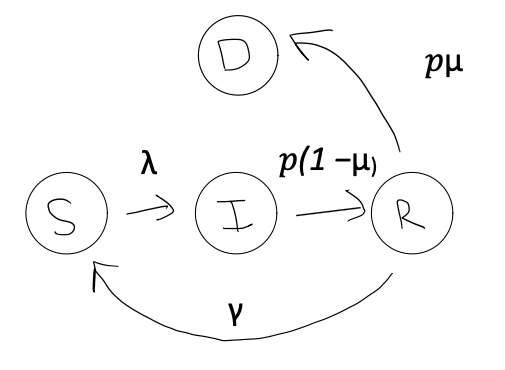
In the above diagram, there are so five transitions possible.
First, $\lambda$ is the force of infection. It combines the chance of getting infected, when meeting someone (which we are setting to 5%) with how often people meet and how many infected people are around. We will represent the chance of getting infected with a $\tau$, for transmission probability. To determine how many people are to be met, and how many of them are infected, we also need to define the size of the population, which we will represent with $N$. The size of the population will repeatedly be adjusted as people drop out (or die) due to the disease, but the initial size of the population will be represented as $N0$.
The more infected people and the more contacts, the higher $\lambda$ becomes, increasing the spread of the disease. The formula for calculating $\lambda$ in this simple example, where we don’t take into account partisan groups or mask wearing, is:
$$ \lambda = \tau c \frac{I}{N} $$
In the above equation, we see that $c$, the average number of contacts, directly increases or decreases $\lambda$.
The number of new infections at in the early phases of the simulation, those people who leave the susceptible class, is therefore calculated as:
$$\text{number of infections} = \frac{dS}{dt} = -S\lambda$$
Now, there is some percentage of people that have ended up as “infected.” Of the infected individuals, we must define how long they will remain in this state. We represent the recovery rate as $\rho$, which is the inverse of the average duration of infectiousness. Specifically:
$$\text{Average duration of infectiousness} = \frac{1} {\rho}$$
In our study, we use $\rho$ = .1, which translates to average duration of infectiousness is 10 time units (days).
To summarize, in order for a transition from $S$ to $I$ to occur, we need a person in state $S$ to come into contact with someone in state $I$. Their probability of transitioning is dependent on $\lambda$, which is calcuted as a combination of transmission probability$\tau$ and average number of contacts $c$. Indirectly, $\lambda$ is impacted by $\rho$, which helps determine the proportion infected at any time $\frac{I}{N}$. To calculate new infections at time t, we multiply $\lambda$ by $S$. A higher $\rho$ leads to faster rate at which individuals leave the infected state which in turns lowers $\lambda$ by reducing the number of infected individuals $I$.
Next, we need to define what happens with people after they’ve become infected. In this case, they can either move into the recovered state or they can die. The transitions are governed by two rates:
$\rho$ - the recovery rate (inverse of the average infectious period) and $\mu$ - the probability of dying following infection.
The rate at which infected individuals move to the deceased state is calculated as $\rho$ times $\mu$ times $I$. In other words, the percentage of infected people who leave the infected state and then die is calculated as:
$$\text{number of deaths} = \frac{dD}{dt} = I\rho\mu$$
Those who do not die transition to the recovered class $R$ at a rate of $\rho$ times $(1-\mu)$ times $I$. This represents the proportion of infected individuals who leave the infected state and recover is calculated as:
$$R = I\rho(1-\mu)$$
Once in the recovered class, just like we observe in COVID-19, individuals lose their immunity and return to the susceptible class at a rate $\gamma$.This represents waning immunity and is calculated as:
$$\text{Rate of Waning Immunity} = R\gamma$$
Now, the overall loop is complete. But, keep in mind that these formulas only represent a single time-step transition. In reality, we are generating these calculations across a set of time units. In our case, we use days and set the default number of days at 250 so we can zoom in on the initial outbreak.
This SIR model implementation uses the deSolve package to numerically solve the system of differential equations over time. The model simulates the progression of the epidemic for each day, updating the state variables (S, I, R) based on the calculated rates of change. This allows us to observe how the epidemic evolves over the specified time period, capturing the dynamics of disease spread, recovery, and the effects of various interventions like vaccination and behavioral changes.
Incorporating Protection (Mask-Usage)
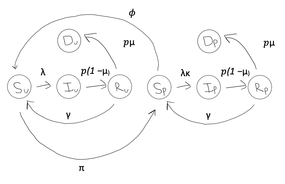
The Berkeley Interpersonal Contacts Study (BICS) showed that Republicans and Democrats report wearing masks at different rates. Since mask-wearing affects disease spread, our model needs to account for these partisan differences. We’ve expanded our basic SIR model to include two new categories: protected ($P$) and unprotected ($U$). This means each state in our model is now split into two. For example, we now have Susceptible Protected ($S_P$) and Susceptible Unprotected ($S_U$), which when added together equal ($S$).
Essentially, the protected class is impacted by s scaling factor $\kappa$, where $\kappa = 1$ means no protection and $\kappa = 0$ perfect protection. Thus, the name “protected” class is a bit of a misnomer if $\kappa$ is not set to 0. Alternatively, we could label it a transmission mitigated class. Thus, for the transmission mitigated class, the force of infection, $\lambda$, is scaled down by a factor $\kappa$. To show this mathematically, we first split the infected class into two groups: $\frac{I}{N} = \frac{I_U}{N} + \frac{I_P}{N}$.
Since $\kappa$ only scales transmission probabilities for the protected, we multiply only against $\frac{I_P}{N}$ so that:
$$\lambda = \tau c (\frac{I_U}{N} + \frac{I_P}{N}\kappa)$$
The above formula implies that contacts with the protected limits an individual’s probability of becoming infected. Of course, the reverse is also true. More contact with the unprotected relatively increases an individual’s probability of becoming infected. However, before becoming infected, the individual also falls into either $S_P$ or $S_U$, which means their probability of becoming infected can become reduced even further. This alters our equation calculating how many people ended as infected for the protected group as:
$$I_P = \frac{dSP}{dt} = -S_P \cdot \lambda \cdot \kappa$$
And those who “choose” not to wear protection effectively remains the same:
$$I_U = \frac{dSU}{dt} = -S_U \cdot \lambda$$
Next, we need a parameter for determining the rate at which people choose to adopt protective behavior. That is, we need a way of transitioning some individuals from the unprotected classes to the protected. For this, we utilize $\pi$, which represents a background rate of adopting protective behavior. It enters our model in the following ways:
First, it reduces the population in $S_U$ at a rate $\pi$ and adds them to $S_P$. But, as we saw during the COVID-19 pandemic, people don’t wear masks forever. We must also incorporate a rate of waning adoption, i.e. a transition of individuals from the protected class back to the unprotected. We will represent this rate as: $\phi$.
$$\frac{dS_U}{dt} = -S_U\cdot\lambda - \pi\cdot S_U + \phi\cdot S_U + \gamma R_U$$
On the other hand (notice $\kappa$):
$$\frac{dS_P}{dt} = -S_P\lambda\cdot\kappa + \pi\cdot S_U - \phi S_U + \gamma R_P$$
In other words, the protected susceptible population ($S_P$) increases as unprotected individuals adopt protective behaviors (at rate $\pi$) and decreases as protected individuals stop using protection (at rate $\phi$). Conversely, the unprotected susceptible population ($S_U$) changes in the opposite direction. Also, at any one point, there are people leaving the recovered classes ($R_U$ and $R_P$) and rejoining their respective susceptible classes. $\pi$ and $\phi$ are also constantly interacting with the other compartments $I$ and $R$, but for the sake of brevity and conciseness I will leave those out of this blog and refer you to the project’s GitHub Repo.
Almost done, but there’s one last component we need to consider: vaccination.
To incorporate vaccination into our model, we move vaccinated individuals directly from the susceptible to the recovered class. This approach assumes that vaccines provide immunity similar to natural infection, with the same waning rate ($\gamma$). The model introduces two key vaccination parameters:
vacc: The daily vaccination rate (e.g., vacc = 0.006 means 0.6% of the population is vaccinated daily)
vstart: The time step when vaccination becomes available
This simplified approach allows us to model the impact of vaccination on disease spread without adding extra compartments, though it doesn’t account for potential differences in immunity between vaccinated and naturally recovered individuals. After we add vaccination, the equations for calculating the susceptible become:
$$\frac{dS_U}{dt} = -(S_U\cdot\lambda) - (\pi\cdot S_U) + (\phi\cdot S_P) + (\gamma \cdot R_U) - (vacc \cdot S_U)$$
$$\frac{dS_P}{dt} = -(S_P \cdot \lambda \cdot\kappa) + (\pi\cdot S_U) - (\phi \cdot S_P) + (\gamma \cdot R_P) - (vacc \cdot S_P)$$
On the other side of the process, the recovered equations become:
$$\frac{dR_U}{dt} = (\rho \cdot (1-\mu) \cdot I_U) - (\pi \cdot R_U) + (\phi \cdot R_P) - (\gamma \cdot R_U) + (vacc \cdot S_U)$$
$$\frac{dR_P}{dt} = (\rho \cdot (1-\mu) \cdot I_P) - (\pi \cdot R_U) - (\phi \cdot R_P) - (\gamma \cdot R_P) + (vacc \cdot S_P)$$
In summary, to account for differences in “protective”, mitigating, behavior, we split up each compartment (S, I, R) into sub-compartments for the protected and unprotected. Most directly, this alters the probability that people in the susceptible class transition into the infected class by altering the equation for $\lambda$. However, indirectly, this impacts the overall pandemic by reducing the proportion of people in the infected class ($I = I_U + I_S$) at any one time, effectively creating a positive feedback loop where $\lambda$ being lower contributes to further declines in $\lambda$ in future states (See equation 1 for the force of infection formula). However, people don’t wear protection forever, and our model reflects that through a parameter $\gamma$ which represents waning adoption. The vaccination rate ($vacc$) and vaccination start time ($vstart$) allows us to transition a percentage of people out of the susceptible compartments and into the recovered compartments, yet they slowly rejoin the susceptible class as their immunity wanes at a rate $\rho$.
Challenge questions:
Why is $(\pi \cdot R_U)$ in our calculation $\frac{dR_P}{dt}$? Why is $(\phi \cdot R_P)$ in our calculation $\frac{dR_U}{dt}$?
How would you draw the $vacc$ parameter onto the flow chart at the beginning of this section? What’s an alternative way to incorporate vaccination?
What is one limitation of the $\kappa$ parameter? What are its assumptions?
How would you calculate the number of people vaccinated at any one point?
Incorporating Groups (Partisans)
After this, incorporating partisanship is relatively easy. As we went over in the previous section, the model extends a standard SIR framework by incorporating both protection status. Each partisan group (Republicans, Democrats, and Independents) is divided into protected and unprotected individuals, creating six distinct subpopulations:
For each partisan group $i \in {a,b,c}$, we track:
Susceptible Population: \(S_{Ui} \text{ (Unprotected)} \quad \text{and} \quad S_{Pi} \text{ (Protected)}\)
Infected Population: \(I_{Ui} \text{ (Unprotected)} \quad \text{and} \quad I_{Pi} \text{ (Protected)}\)
Recovered Population: \(R_{Ui} \text{ (Unprotected)} \quad \text{and} \quad R_{Pi} \text{ (Protected)}\)
Where:
- $i = a$: Republicans
- $i = b$: Democrats
- $i = c$: Independents
The model tracks these compartments simultaneously with group-specific parameters:
- Protection adoption rate: $\pi_i$ -Contact rate: $c_i$
- Mortality rate: $\mu_i$
Using republicans as an example, we would calculate the rate of change in the susceptible class like this:
For "unprotected" Republicans: $$\frac{dS_{Ua}}{dt} = -(S_{Ua} \cdot \lambda_a) - (\pi_a\cdot S_{Ua}) + (\phi_a \cdot S_{Pa}) + (\gamma \cdot R_{Ua}) - (vacc_a \cdot S_{Ua})$$ And for the "protected" Republicans: $$\frac{dS_{Pa}}{dt} = -(S_{Pa} \cdot \lambda_a \cdot \kappa) + (\pi_a \cdot S_{Ua}) - (\phi_a \cdot S_{Pa}) + (\gamma \cdot R_{Pa}) - (vacc_a \cdot S_{Pa})$$
These two groups make up the susceptible compartment for the Republican group. Notice here that every parameter except for $\gamma$ and $\kappa$ is being assigned a subscript a. This is because $\gamma$ is the rate of waninng immunity, and we aren’t expecting that to vary by party affiliation. As for $\kappa$, which represents the effectiveness of “protection,” It’s quite possible that Democrats, for example, are wearing protection that is more effective than Republicans. For example, we know that N95 masks are more effective at reducing transmission than cloth masks. However, for this early iteration of the model, we will keep it simple and calculate one value for $\kappa$.
Further, survey data from BICS shows that Republicans, Democrats, and Independents adopt protective behaviors like mask-wearing at different rates. To capture this variation, each group needs to have its own protection adoption rate ($\pi$) and protection waning rate ($\phi$). These group-specific rates reflect the real-world differences in how quickly each partisan group takes up and abandons protective measures.
But why does $\lambda$ change based on partisan group? The force of infection varies by partisan group because it depends not just on how many contacts someone has, but who those contacts are and their protection status. Since protection rates differ by party, we must account for both the quantity and partisan composition of contacts. For example, if Republicans primarily interact with other Republicans who are less likely to be protected, their force of infection ($\lambda_a$) will naturally differ from Democrats who might mainly contact other Democrats with higher protection rates. This interaction between social mixing patterns and group-specific protection rates creates distinct transmission dynamics for each partisan group. For example, for Republicans, we calculate force of infection as:
$$\lambda_a = \tau \left( c_{a,a} \left(\frac{I_{Ua}}{N_a} + \kappa\frac{I_{Pa}}{N_a}\right) + c_{a,b} \left(\frac{I_{Ub}}{N_b} + \kappa\frac{I_{Pb}}{N_b}\right) + c_{a,c} \left(\frac{I_{Uc}}{N_c} + \kappa\frac{I_{Pc}}{N_c}\right) \right)$$
There’s a lot going on here, so let’s break it down step-by-step. Frst, notice that the transmission probablity ($\tau$) is constant and doesn’t have a subscript. This is because the transmission probability is a feature of the virus, which doesn’t stop to consider your political affiliation before it infects you. Next, instead of just $c$ (contacts) we now have:
- $c_{a,a}$: Republican contacts with Republicans
- $c_{a,b}$: Republican contacts with Democrats
- $c_{a,c}$: Republican contacts with Independents
Each contact rate is multiplied by the proportion of infected individuals in the corresponding group. Therefore, $\lambda_a$ increases with both the frequency of contacts and the infection levels within contacted groups. On the other hand, it decreases when contacts switch from a group that’s highly infected to a group that’s less infected (due to some combination of lower contacts or lower mask usage). We could also see this as three distinct $\lambda$ parameters, or:
$$\lambda_a = \lambda_{a,a} + \lambda_{a,b} + \lambda_{a,c}$$
Let’s move on to the infected.
$$ \frac{dI_{Ua}}{dt} = (S_{Ua} \cdot \lambda_a) - (\pi_a \cdot I_{Ua}) + (\phi_a \cdot I_{Pa}) - (\rho \cdot I_{Ua}) $$ $$ \frac{dI_{Pa}}{dt} = (S_{Pa} \cdot \kappa \cdot \lambda_a) + (\pi_a \cdot I_{Ua}) - (\phi_a \cdot I_{Pa}) - (\rho \cdot I_{Pa}) $$
Calculating those in the the rate of change in the recovered class is done like this:
$$\frac{dR_{Ua}}{dt} = (\rho \cdot (1-\mu_a) \cdot I_{Ua}) - (\pi_a \cdot R_{Ua}) + (\phi_a \cdot R_{Pa}) - (\gamma \cdot R_{Ua}) + (vacc_a \cdot S_{Ua})$$
Notice here that features of the disease remain the same, but anything that involves differences in behavior are assigned a unique subscript a, b, or c. This means $mu$ gets a subscrupt $mu_a, because the probability of dying is partially a consequence of age, and partisan groups tend to differ along average age.